Statistical Nature of Light
One of the fundamental concepts in image sensors is the statistical nature of light, and the fact that photo-detectors receive and integrate individual photons. The statistics of photon arrival are unavoidable, and the noise present in the light itself has to be accepted. The noise in the light is called photon shot noise and even a perfect detector is subject to it.
Poisson Process
In most cases, a light source can be modeled using a Poisson process. The Poisson process describes a series of random events which satisfy the following three conditions:
Every event is independent i.e. the process is memoryless.
The average rate of events is constant.
Two events cannot occur at the same time.
An illustration of the random events from a Poisson process are plotted below. The plot shows 50 events drawn from a Poisson process with an average rate of 10.
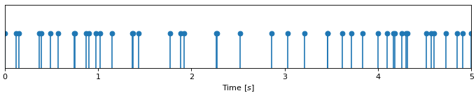
The plot resembles the output of a single photon detector.
Video explanation of the Poisson Process
Poisson Distribution
For a random variable \(X\) described by a Poisson process where the average number of events in a given interval is equal to \(\lambda\), the probability of \(k\) events occurring in any individual interval is given by the Poisson distribution:
The length of the interval of interest doesn’t really matter in this description, however in an image sensor context it is convenient to think of it as the expected number of photons collected during an exposure, therefore it can be broken down into
The distribution has an interesting property, in that its expected value (mean) is equal to its variance
which makes the standard deviation of this distribution
A plot of the distribution with various rate parameters looks like this:
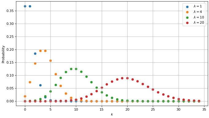
Probability mass function of the Poisson distribution.
Exponential Distribution
The time between consecutive events in a Poisson process can be described by the exponential distribution. This is actually a consequence of the memoryless property [1] [2]
The exponential distribution is described by the following
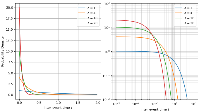
The exponential distribution plotted on linear axes (left) and on log-log axes (right)
This distribution can be used to find the probability of at least 1 photon arriving in a given time window \(T\). This is the same as the probability of the photon arriving before time \(T\), and equivalent to no photons arriving before time \(T\). Mathematically this is expressed by
This distribution can be sampled from if you want to generate a stream of photon events in the time domain.
Photon Shot Noise
Photon shot noise is the name given to the noise seen by a photodetector due to the natural statistical variations in the light itself.
The Poisson distribution is useful in predicting the photon shot noise, which is the dominant noise source at high illumination levels. For example a perfect detector which captures \(N=10,000\) photo-electrons, and which has no read noise will have a noise level equal to \(\sqrt{N}=100\)
Signal to Noise Ratio
The signal and noise levels can be combined in one value which expresses a general quality of an image. Considering only the photon shot noise in this example we can write
If instead of \(N\) we substitute the full well capacity of a detector we actually obtain the an expression for the maximum signal to noise ratio as the noise in the light will become the limiting factor.
This expression for SNR is the output referred SNR because to calculate it only the signal and noise at the output are needed. It is a good approximation in cases where the signal \(N\) is thousands of photo-electrons, but does not hold when the signal is low. In such cases the complete exposure referred SNR [3] expression should be used.
The above can be re-written as
In the above \(\theta\) is the exposure given by the photon rate multiplied by the exposure time. \(Y\) is a random variable which represents the number of counted photo-electrons. It behaves like the random variable \(X\) (see above) but is bounded by the full well capacity \(L\) of the detector which is just an non-zero integer. It can be considered to be a truncated Poisson distribution with \(\mu\) being its expected value.
The probability mass function of \(Y\) is then
The sum to infinity, which is the tail of the Poisson distribution, can be conveniently calculated using the incomplete gamma function . When plotted this truncated Poisson distribution looks like this
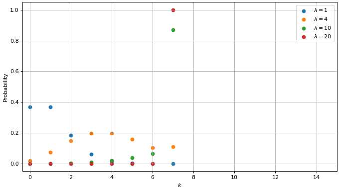
The truncated Poisson distribution with a limit \(L\) of 7, for different event rates.
Note how in this case when \(\lambda = 4\) the probability of counting 6 and 7 events is almost the same, and when \(\lambda = 20\) the count will reach the limit almost 100% of the time.
The output referred SNR is related to the exposure referred SNR by the following